Long Term Trends In College Education And Income: 1960 - 2015

Part I of a two part series on college education. Part I discusses long term trends in average income outcomes. Part II will discuss the heterogeneity of college outcomes related to income and upward mobility.
Summary:
- In 1960, 50% of the top income quintile for 32 - 34 year olds had a high school education or less. By 2015 that percentage shrank to 9%.
- The correlation between having a 4 year college degree and achieving high relative income has weakened since 1960 because the percentage of workers with a 4 year college degree or graduate degree increased from 12% to 40% by 2015.
- For the US as a whole, real median Inflation adjusted income has only grown for those with graduate degrees.
Data
The data used here is US Census data made available by IPUMS.org.[1] Following the methodology of Chetty, Friedman, Saez, Turner, and Yagan in their 2017 paper: “Mobility Report Cards: The Role of Colleges in Intergenerational Mobility”, this analysis focuses on 32-34 year olds. While income is strongly related to age, lifetime relative income rank is relatively stable by the time workers reach their early 30s. Thus when I refer to upper income quintile, I am referring to the upper income quintile of 32-34 year olds -- not to the entire US population.
While later Census surveys distinguished between different levels of graduate degrees, in 1960 the three highest educational categories were “4 years of college”, “5 years of college”, and “6+ years of college.” I conform these categories with later surveys by grouping 4 years and 5 years together as “Bachelor’s” and classify “6+ years” as “More Than Bachelor's.” For later surveys, Masters and PhDs are classified together as “More Than Bachelor’s.” As a shorthand, I will refer to “More Than Bachelor’s” as those with “graduate degrees” and those with “Bachelor’s” as those with “undergraduate degrees.” My category “Some College” includes those who receive two-year degrees.
To concentrate on US college experience and its impact on employment income, this analysis is limited to US born workers with positive wage income. My use of the word “income” excludes all other sources of income as I focus on education’s relation to wages (e.g., not savings behavior, inheritance etc.).
My focus on only those with wage income understates the overall social impact of education on income because those without any college education are less likely to earn wages. The percent of 32-34 year olds with High School or less that had wage income rose from 61% in 1960 to 69% in 2015. That compares to 73% in 1960, and 90% in 2015 for those with 4 years of college or more. Increased female labor force participation increased the percentage of those employed across all education levels over this time period, however it only increased by 8% for those with High School or less versus by 17% for those with 4 years of college or more.[2]
Upper Income Quintile Share
Figure 1 shows the share of the upper income quintile by educational attainment. The share of those with High School and less than High School education declined sharply over this period. The largest increase in relative share was for those with graduate degrees.
Figure 1: Long Term Trends In Upper Income Quintile Share By Education

Increased Supply of College Educated Labor
Figure 2 shows the share of workers by educational attainment. The share of all workers with an undergraduate degree increased from 10% to 25% over this period. The share with graduate degrees increased from 2% to 14%. The percentage with High School remained relatively constant, dropping from 29% to 23%. Notably, in 2015 73% of all workers had some college education.
Figure 2: Long Term Trends In Worker Share By Education

The Implication Of Increased Supply For The Probability Of Upper Income
Because there were relatively few workers with undergraduate and graduate degrees in 1960, the likelihood of achieving the top income quintile if you had one of those degrees was quite high: 50% for undergraduates and 54% for graduates. By 2015, those probabilities had dropped to 32% for undergraduates, and less dramatically to 44% for those with graduate degrees. Note that these probabilities don’t sum to 100% -- if everyone had the same educational attainment, the probability for all would be 20%.
Figure 3: Long Term Trends In Probability Of Upper Income Quintile By Educational Attainment

The Implication Of Increased Supply Of College Educated Workers For Relative Income And Real Income Growth
Theoretically wages are a function of both the supply of labor at a particular “skill level” and demand for that “skill level.” Demand is related to industrial mix (e.g., the share of knowledge-based industries) and the value that a given “skill level” is capable of producing.
For example in an economy where all employment opportunities involved manual labor, demand for PhDs would be low (and they would have no wage advantage) because their additional education provides no incremental value for that set of employment opportunities.
For example in an economy where all employment opportunities involved manual labor, demand for PhDs would be low (and they would have no wage advantage) because their additional education provides no incremental value for that set of employment opportunities.
Similarly, if the government decided to provide every citizen with a college education but the mix of job types in the economy did not change, there would be a lot of college educated waiters, auto mechanics, construction workers etc. In this hypothetical case there is little reason to think a "universal college" social policy would change income outcomes. In this context, it is worth noting that the US already has the 7th highest percentage of "tertiary education" among 44 countries followed by the OECD.
To further complicate matters, labor supply has become increasingly global (so US-based Figure 2 does not accurately represent the true labor supply available to producers). Labor also competes with capital in the form of automation.
Given the complexity of global labor supply and automation, it is difficult to link US real wages by educational attainment solely to increases in the supply of US college educated workers. We can simply observe growth in absolute and relative real wages to infer the economic value of educational attainment.
Figure 4: Median Income in 1960 Dollars By Education For 32-34 Year Old Workers

Figure 4 shows an increasing gap between those who have an undergraduate or graduate degrees and those that don’t. That is, education has increased income on a relative basis for those with 4 years of college or more. However this relative improvement is primarily due to the deterioration in the real income of those with less than a 4 year degree.
Figure 4 also shows that only those with graduate degrees have seen any real growth in median income since 1960. At a broad level, this suggests the still relatively small supply of those with graduate degrees and their productivity in the context of the current US economy has been enough to offset competition from increased automation and global labor competition.
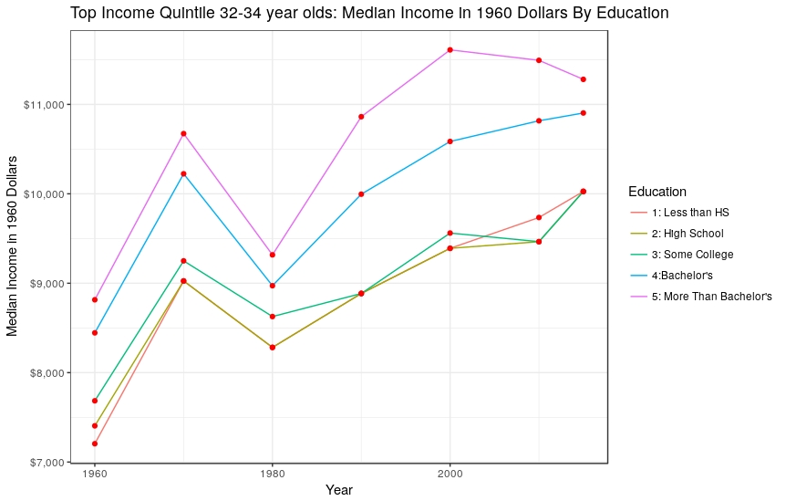
Real income growth has been strongest for those in the top income quintile as shown in Figure 5. This is true regardless of education and is probably related to the increasing ability to leverage ability/aptitude in certain fields via technology. Examples would include the increased media value of elite athletes and increased productivity of those working in high tech fields. We will see in Part II of this analysis that the percentage of STEM majors by college has a statistically significant correlation with 32-34 year old incomes by college.
Figure 5: Median Income in 1960 Dollars For 32-34 Year Old Workers In The Top Income Quintile By Education
Averages Don’t Capture Significant Differences In Outcome By College
The broad averages shown in Figures 1 - 5 mask the fact that outcomes for individual students vary significantly by college. Table 1 uses 2014 data from the Chetty, Friedman, Saez, Turner, and Yagan paper described above for students who attended college from 1999 - 2004. This is a sub-sample of their data based on 1,208 colleges not identified as “Two-Year” colleges with a cohort size of more than 150 students.[3] The table shows the weighted (by number of students per college) median fraction of students who achieve the top income quintile when they are 32-34 years old by Barron’s Selectivity Index.
Notably these success rates include students who go on to get graduate degrees (so they resemble a blend of the 32% undergraduate and 44% graduate probabilities for 2015 described above).
Table 1: 2014 Probability Of Being In Top Income Quintile For 32-34 Year Olds Who Attended A 4 Year College By Barron’s College Selectivity Index
Barron's Selectivity Index
|
Weighted Median of Probability of Top Income Quintile For Colleges In Category
|
Share of Students In Sub-Sample
|
Cum. Share Of Students
|
Elite
|
61%
|
6.3%
|
6.3%
|
Highly Selective
|
51%
|
14.0%
|
20.3%
|
Selective +
|
40%
|
23.5%
|
43.8%
|
Selective
|
30%
|
34.6%
|
78.5%
|
Selective-
|
24%
|
10.1%
|
88.5%
|
Special
|
25%
|
0.8%
|
89.3%
|
Non-Selective
|
17%
|
10.7%
|
100.0%
|
Also shown are the share and cumulative share of students by category for this sub-sample. There is marked divergence between the 17% top income quintile probability for the 11% of students who attended “Non-Selective” colleges versus the 61% top income quintile probability for the 6% of students who attended “Elite” colleges.
Part II of this analysis will examine the characteristics of colleges that are correlated with these widely divergent outcomes.
[1] Data available from IPUMS-USA, University of Minnesota, www.ipums.org. It is freely available subject to their licensing agreement.
[2] The increase in educated female labor force participation has also contributed to rising income inequality at the household level.
[2] The increase in educated female labor force participation has also contributed to rising income inequality at the household level.
[3] See their paper for details regarding cohort sizes and a description of their variable “College Tier Name.”
Transparent and reproducible: All Figures and Tables can be generated by using the free, publicly-available R program and the R code available in “degreeShare.r" on github to analyze the publicly available data obtainable from the links in the article.


Comments